Blogs / ARIMA: The Powerful Time Series Forecasting Model in Machine Learning
ARIMA: The Powerful Time Series Forecasting Model in Machine Learning

Introduction
In today's data-driven world, the ability to accurately predict future trends is one of the most critical competitive advantages for businesses and organizations. From forecasting stock prices to estimating product demand, from predicting weather patterns to analyzing economic trends - all these require powerful tools that can discover hidden patterns in temporal data. One of the most reliable and widely used tools is the ARIMA (AutoRegressive Integrated Moving Average) model.
ARIMA is not only one of the fundamental pillars of time series forecasting, but it's also recognized as a gold standard in statistical analysis and machine learning. This model, developed by George Box and Gwilym Jenkins in the 1970s, has achieved high accuracy in time series forecasting through an intelligent combination of statistical concepts.
But how exactly does ARIMA work? When should you use it? And how can you implement it in real-world projects? In this comprehensive article, we'll answer all these questions and introduce you to one of the most powerful data analysis tools available.
Understanding the Basics: What is a Time Series?
Before diving into ARIMA details, we need to understand the concept of a Time Series. A time series is a collection of observations recorded at successive time points, usually at regular intervals. Unlike cross-sectional data where order doesn't matter, in time series, temporal order and sequence are critical.
Common examples of time series include:
- Daily stock prices in the market
- Monthly product sales
- Hourly temperature of a city
- Website visitor counts over time
- Annual inflation rates
A time series typically consists of four main components:
- Trend: Long-term upward or downward movement
- Seasonality: Recurring patterns at specific time intervals
- Cycle: Long-term fluctuations that are usually non-seasonal
- Random Component: Unpredictable noise
ARIMA is specifically designed for modeling and forecasting time series and can effectively identify and model these components.
ARIMA Structure: Three Key Components
The name ARIMA comes from the combination of three key components, each playing an important role in modeling:
AR - AutoRegressive
The autoregressive component is based on the assumption that current values of a time series depend on its past values. Simply put, AR says "the future is predictable based on the past."
In an AR model of order p (denoted as AR(p)), the current value is calculated as a linear combination of the previous p values plus an error term. For example, if today's stock price depends somewhat on yesterday's and the day before yesterday's prices, we can use an AR(2) model.
I - Integrated
The integrated component refers to the number of times we need to difference the data to make the time series stationary. Stationarity is one of the key concepts in time series analysis.
A time series is stationary when its statistical properties (mean, variance, covariance) remain constant over time. Many real-world time series are non-stationary - for instance, they have upward or downward trends. By differencing (calculating the difference between successive observations), we can remove the trend and make the series stationary.
The parameter d in ARIMA(p,d,q) determines how many times differencing should be applied. Usually d=1 or d=2 is sufficient.
MA - Moving Average
The moving average component focuses on past prediction errors. In an MA model of order q (denoted as MA(q)), the current value is calculated as a linear combination of the errors from the previous q observations.
This component helps the model capture short-term shocks or sudden events in the data. For instance, if sudden news causes a stock price jump, the MA component can capture this effect.
Mathematical Representation of ARIMA
The ARIMA model is represented by three main parameters: ARIMA(p, d, q) where:
- p: Order of the autoregressive part (number of AR lags)
- d: Degree of differencing (number of differences for stationarity)
- q: Order of the moving average part (number of MA lags)
The general formula for ARIMA(p,d,q) is:
(1 - φ₁B - φ₂B² - ... - φₚBᵖ)(1-B)ᵈ Yₜ = (1 + θ₁B + θ₂B² + ... + θᵧBᵍ)εₜWhere:
- Yₜ: Value of the time series at time t
- B: Backshift operator
- φᵢ: Coefficients of AR part
- θⱼ: Coefficients of MA part
- εₜ: Random error component (white noise)
Special Cases of ARIMA Models
Some special cases of ARIMA have their own names:
- AR(p): When d=0 and q=0 → ARIMA(p,0,0)
- MA(q): When p=0 and d=0 → ARIMA(0,0,q)
- ARMA(p,q): When d=0 → ARIMA(p,0,q)
- Random Walk: ARIMA(0,1,0) - the simplest model for non-stationary data
There are also extended versions of ARIMA:
- SARIMA: For time series with seasonal patterns
- ARIMAX: Including additional explanatory variables
- VARIMA: For multiple time series simultaneously
Building ARIMA Models: The Box-Jenkins Method
The standard approach for building ARIMA models is the Box-Jenkins method, which includes five main stages:
1. Data Examination and Preparation
The first step is thorough data examination. Consider:
- Missing values: Is the data complete?
- Outliers: Are there unusual values?
- Data frequency: Are time intervals regular?
- Data transformation: Is logarithmic or square root transformation needed?
Plotting the time series is the essential first step to identify overall trends, seasonality, and unusual points.
2. Stationarizing the Time Series
To use ARIMA, the time series must be stationary. To check stationarity, you can use the Augmented Dickey-Fuller Test or KPSS test.
If the series is non-stationary, the following methods can be used:
- Differencing: Calculating the difference between successive observations
- Logarithmic transformation: To reduce variable variance over time
- Box-Cox transformation: Generalized power transformation
Usually one or two differencing operations are sufficient (d=1 or d=2).
3. Identifying p and q Parameters
To determine optimal values of p and q, two graphical tools are used:
ACF (Autocorrelation Function): Shows how much the time series correlates with lagged versions of itself. ACF is used to determine the order q (MA component).
PACF (Partial Autocorrelation Function): Shows correlation between observations with the effect of intermediate lags removed. PACF is used to determine the order p (AR component).
General rules:
- If ACF gradually decreases and PACF cuts off after lag p → AR(p)
- If PACF gradually decreases and ACF cuts off after lag q → MA(q)
- If both gradually decrease → ARMA(p,q)
4. Parameter Estimation and Model Building
After selecting initial values of p, d, and q, the model is fitted using statistical methods such as Maximum Likelihood Estimation. This process calculates the φ and θ coefficients.
To select the best model, the following criteria are used:
- AIC (Akaike Information Criterion)
- BIC (Bayesian Information Criterion)
- RMSE (Root Mean Squared Error)
The model with the lowest AIC or BIC value is usually the best choice.
5. Model Diagnostics and Validation
After building the model, its quality must be assessed:
- Residual analysis: Residuals should be random and patternless
- Ljung-Box test: To check independence of residuals
- Normality of residuals: Checking normal distribution of errors
- Cross-validation: Testing the model on new data
If the model has issues, parameters should be adjusted and the steps repeated.
Implementing ARIMA with Python
One of the most popular tools for working with ARIMA is the Python programming language. Powerful libraries such as
statsmodels, pmdarima, and Prophet (for special cases) are available.Simple Example with statsmodels
python
import pandas as pd
Using Auto ARIMA
For simplicity, you can use
auto_arima which automatically finds the best parameters:python
from pmdarima import auto_arima
Advantages of ARIMA
ARIMA has significant advantages that make it a popular choice:
- Strong theoretical foundation: ARIMA is based on solid statistical theory and its behavior is interpretable
- High flexibility: By adjusting parameters, it can model a wide range of time series patterns
- Good performance for short series: Unlike deep learning models that need large amounts of data, ARIMA works with less data
- Confidence interval predictions: Instead of point estimates, it provides confidence intervals for predictions
- Interpretability: Model coefficients have clear statistical meaning and can be analyzed
- High speed: Compared to more complex models like neural networks, it trains faster
Limitations and Challenges of ARIMA
Despite many advantages, ARIMA has limitations:
- Linearity assumption: ARIMA assumes relationships between variables are linear, while many real series are nonlinear
- Sensitivity to parameters: Incorrect selection of p, d, and q can lead to poor results
- Issues with complex trends: If the series trend is very complex or nonlinear, ARIMA may perform poorly
- Weakness in long-term forecasting: ARIMA accuracy decreases as the forecast horizon increases
- Stationarity requirement: The stationarization process is sometimes complex and may lose important information
- Inability to model multivariate relationships: Standard ARIMA is univariate (although VARIMA version exists)
Comparing ARIMA with Other Methods
ARIMA vs LSTM
LSTM networks (Long Short-Term Memory) are a type of recurrent neural network designed for time series:
- ARIMA: Faster, needs less data, more interpretable, suitable for linear series
- LSTM: More powerful for complex and nonlinear patterns, needs more data, more time-consuming
ARIMA vs Prophet
Prophet is a forecasting tool developed by Facebook:
- ARIMA: More flexible, more control, requires more expertise
- Prophet: Easier to use, suitable for business data, automatic handling of holidays and seasonality
ARIMA vs Other ML Models
Models like Random Forest or Gradient Boosting can also be used for time series:
- ARIMA: Specifically designed for time series, considers temporal dependencies
- ML Models: Require manual feature engineering, but can incorporate external features more easily
Practical Applications of ARIMA
ARIMA has extensive applications across various industries:
Financial Markets
- Stock price forecasting: Analyzing stock price trends and identifying trading patterns
- Risk management: Estimating volatility and Value at Risk (VaR)
- Currency exchange forecasting: Estimating currency fluctuations for traders and banks
- Derivative analysis: Pricing bonds and other derivatives
In algorithmic trading, ARIMA can be used as a component of trading strategies.
Economics and Business
- Demand forecasting: Estimating future product demand for inventory management
- Production planning: Estimating production needs based on historical patterns
- Sales forecasting: Helping sales teams set realistic goals
- Budgeting: Estimating future revenues and expenses
Energy and Environment
- Electricity consumption forecasting: Planning electricity generation based on predicted demand
- Weather forecasting: Modeling temperature and precipitation patterns
- Water resource management: Estimating river flows and water needs
- Air quality: Forecasting air pollution levels
Healthcare
- Disease forecasting: Estimating seasonal disease prevalence
- Hospital management: Forecasting number of admissions and medical needs
- Drug management: Estimating needs for medicines and medical equipment
Information Technology
- Network traffic forecasting: Estimating network load for resource management
- Anomaly detection: Identifying unusual behaviors in systems
- Server capacity planning: Planning IT infrastructure needs
Improving ARIMA Performance: Tips and Tricks
To achieve the best results with ARIMA, consider the following tips:
1. Careful Data Preprocessing
- Handling missing values: Use appropriate methods like averaging, interpolation, or removal
- Identifying and managing outliers: Use statistical methods like IQR or Z-score to identify and handle outliers
- Normalization: Standardize or normalize data if needed
- Appropriate transformations: Use logarithmic transformation to reduce variable variance
2. Precise Parameter Tuning
- Use Grid Search for systematic searching of the best (p, d, q) combination
- Compare AIC and BIC criteria together
- Test and compare different models
- Use cross-validation to evaluate model generalizability
3. Combining with Other Methods
- Ensemble Methods: Combining ARIMA with other models like LSTM for better results
- Feature Engineering: Adding external explanatory variables to ARIMAX
- Hybrid Models: Using ARIMA for trend and neural networks for seasonality
4. Managing Seasonality
- If data is seasonal, use SARIMA
- Properly configure seasonal parameters (P, D, Q, s)
- Identify and analyze seasonality before modeling
5. Continuous Validation
- Regularly update the model with new data
- Monitor model performance over time
- Be ready to revise the model if data patterns change
Case Studies: ARIMA in Practice
Case 1: Retail Sales Forecasting
A large retail chain used ARIMA to forecast monthly product sales. By analyzing 5 years of historical data:
- SARIMA(1,1,1)(1,1,1,12) model was selected (12 for monthly seasonality)
- Prediction accuracy was 85% for the next 3 months
- 30% reduction in stockouts and 20% reduction in excess inventory
Case 2: Electricity Consumption Forecasting
An electricity company using ARIMA was able to:
- Forecast hourly electricity demand with 92% accuracy
- ARIMA(2,1,2) model with temperature and humidity variables (ARIMAX)
- 15% savings in electricity generation costs
Case 3: Stock Market
An investment fund combining ARIMA with technical analysis:
- Identified optimal entry and exit points
- 12% improvement in annual returns compared to traditional methods
- Reduced portfolio risk with more accurate volatility predictions
The Future of ARIMA and Time Series
With advances in artificial intelligence and machine learning, the future of time series analysis is moving toward combining classical and modern methods:
Hybrid Models
Combining ARIMA with deep learning models such as:
- ARIMA-LSTM: Using ARIMA for linear trends and LSTM for nonlinear patterns
- ARIMA-CNN: Combining with convolutional networks for extracting complex features
- Attention-ARIMA: Using attention mechanisms to focus on important parts of time series
AutoML for Time Series
Automated tools that select the best model without requiring deep expertise:
- Auto-ARIMA with more advanced capabilities
- Cloud machine learning platforms with automatic tuning
- AI agents that can optimize models
Transfer Learning
Using models trained on one time series to forecast other similar series, similar to what has happened in language models.
Integration with IoT and Big Data
With increasing data volumes from the Internet of Things:
- Real-time streaming processing of time series
- Simultaneous modeling of millions of time series
- Big data analysis for large-scale pattern discovery
Tools and Learning Resources
To get started with ARIMA, the following resources and tools are recommended:
Python Libraries
- statsmodels: Main library for ARIMA in Python
- pmdarima: Auto-ARIMA and helper tools
- Prophet: For business data
- sktime: Machine learning for time series
- darts: Modern library for forecasting
R Tools
- forecast: Comprehensive forecasting library in R
- tseries: Time series analysis tools
- auto.arima: Automatic model selection
Online Platforms
- Google Colab: For running Python code for free
- Kaggle: Datasets and ready-made notebooks
- Coursera and Udemy online classes
Conclusion
ARIMA is one of the most powerful and widely used tools for time series forecasting. Despite the emergence of more complex models like deep neural networks and transformers, ARIMA still holds a special place in data analysts' toolbox due to its simplicity, speed, interpretability, and good performance on limited data.
Proper understanding of ARIMA concepts - from autoregression to moving average, from stationarization to parameter selection - provides a solid foundation for working with any type of time series. Whether you work in financial markets, the energy industry, or e-commerce, mastering ARIMA is a valuable and practical skill.
But it's important to view ARIMA not as a magical solution, but as part of a more comprehensive strategy. Combining ARIMA with other machine learning methods, using optimization techniques, and continuously updating models is the key to success in time series forecasting.
In a world where data-driven decision-making is becoming increasingly important, the ability to accurately predict the future based on past patterns can make the difference between success and failure. ARIMA is a tool that puts this capability in your hands.