Blogs / Time Series Forecasting with Artificial Intelligence: From Basics to Practical Implementation
Time Series Forecasting with Artificial Intelligence: From Basics to Practical Implementation

Introduction: Why Time Series Forecasting Matters
In today's world, strategic decision-making for businesses and organizations heavily relies on accurate future predictions. From forecasting product sales to analyzing financial markets, from warehouse inventory management to energy consumption planning - all these areas require understanding temporal patterns and predicting future trends.
Time Series Forecasting is the science and art of predicting future values based on past observations. With the emergence of artificial intelligence and machine learning, this field has undergone a profound transformation. Modern AI models can discover complex patterns that traditional methods couldn't identify and use them for more accurate predictions.
In this comprehensive article, we'll deeply explore concepts, algorithms, tools, and practical techniques for time series forecasting with artificial intelligence, and guide you step-by-step through implementing real-world projects.
What is Time Series? Basic Concepts
A Time Series is a collection of data points recorded at specific and usually regular time intervals. Each data point belongs to a specific time, and the temporal order of these data points is extremely important.
Main Components of Time Series
Every time series typically consists of four main components:
1. Trend: The general direction of data movement over time. Trends can be upward, downward, or stable. For example, population growth or increasing sales of a successful product.
2. Seasonality: Repeating patterns at fixed time intervals. For instance, increased winter clothing sales during cold seasons or increased website traffic at specific hours of the day.
3. Cyclicality: Long-term fluctuations that don't repeat regularly and are usually related to economic or business factors.
4. Noise/Residual: Random and unpredictable fluctuations that remain after removing the previous three components.
Important Time Series Properties
To work with time series and choose the appropriate model, you need to be familiar with some key concepts:
Stationarity: A time series is stationary when its statistical properties (mean, variance) remain constant over time. Many traditional models require stationary data.
Autocorrelation: The degree of correlation of a time series with itself at different time lags. This property helps identify repeating patterns.
Lag: The time distance between observations. For example, comparing today's sales with sales from one week ago.
Why AI for Time Series Forecasting?
Traditional statistical methods like ARIMA, Exponential Smoothing, and other classical techniques have been used for decades in time series forecasting. However, these methods have limitations:
- Inability to identify complex nonlinear patterns
- Need for manual preprocessing and precise parameter selection
- Poor performance with multivariate data
- Limitations in managing long-term dependencies
Deep learning and AI models have addressed these limitations:
✅ Automatic feature learning: No need for manual feature extraction
✅ Complexity management: Ability to model nonlinear and complex relationships
✅ Scalability: Working with massive data volumes
✅ Multivariate capability: Simultaneous use of multiple related time series
✅ Flexibility: Adaptability to various types of data and patterns
AI Models for Time Series Forecasting
1. Recurrent Neural Networks (RNN)
Recurrent Neural Networks were the first generation of deep learning models for time series. These networks have feedback loops that preserve information throughout the sequence.
Advantages:
- Ability to process variable-length sequences
- Short-term memory for retaining previous information
Disadvantages:
- Vanishing or exploding gradient problem
- Inability to learn long-term dependencies
- Slow and expensive training
2. Long Short-Term Memory (LSTM)
LSTM is an improved version of RNN that solves its main problems. LSTM can preserve important information for long periods using special gates (forget, input, output).
LSTM Structure:
- Forget Gate: Decides what information to remove from cell memory
- Input Gate: Determines what new information to add to memory
- Output Gate: Determines what part of memory to transfer to output
Practical Applications:
- Stock price and cryptocurrency prediction
- Energy demand forecasting
- Sales trend analysis and prediction
3. Gated Recurrent Units (GRU)
GRU is simpler than LSTM but performs similarly. This architecture has only two gates (update and reset) and requires fewer parameters to train.
Advantages over LSTM:
- Faster training speed
- Less memory requirement
- Similar performance in many applications
When to choose GRU?
- Smaller datasets
- Need for faster training
- Limited computational resources
4. Transformer-Based Models
The Transformer architecture, originally designed for natural language processing, has revolutionized time series forecasting.
Temporal Fusion Transformers (TFT): This model combines LSTM and attention mechanism, capable of:
- Processing multiple variables simultaneously
- Identifying relative importance of each variable
- Providing high interpretability
Informer and Autoformer: More advanced models designed for long time series that use optimized attention mechanisms.
5. Hybrid and Advanced Models
Prophet: A model developed by Meta designed for businesses. This model:
- Can be used without deep expertise
- Works well with incomplete data
- Manages multiple seasonalities
- Considers holidays and special events
N-BEATS: A pure neural architecture based on stacked blocks that works without feature extraction.
DeepAR: Amazon's probabilistic model suitable for group forecasting of multiple related time series.
Practical Steps for Time Series Forecasting
Step 1: Data Collection and Exploration
The first and most important step is preparing quality data. Your time series data should:
- Be complete and without gaps (or gaps properly managed)
- Have accurate timestamps
- Be recorded at constant frequency (e.g., daily, hourly)
- Be collected from reliable sources
For initial data exploration, use the pandas library:
python
import pandas as pd
Step 2: Data Preprocessing and Preparation
Handling Missing Values:
python
# Different methods for filling missing values
Identifying and Handling Outliers:
python
from scipy import stats
Data Normalization:
python
from sklearn.preprocessing import MinMaxScaler, StandardScaler
Time Series Decomposition:
python
from statsmodels.tsa.seasonal import seasonal_decompose
Step 3: Feature Engineering
Good features can dramatically improve model performance:
Temporal Features:
python
df['year'] = df.index.year
Lag Features:
python
# Create lag features
Rolling Window Features:
python
# Rolling average
Step 4: Data Splitting for Training and Evaluation
In time series, you should not use random splitting. You must preserve temporal order:
python
# Simple time split
Step 5: Building and Training the Model
Example 1: LSTM Implementation with TensorFlow/Keras
python
from tensorflow import keras
Example 2: Using Prophet
python
from prophet import Prophet
Step 6: Model Evaluation
Various metrics are used to evaluate time series forecasting model performance:
Mean Absolute Error (MAE):
python
from sklearn.metrics import mean_absolute_error
Root Mean Squared Error (RMSE):
python
from sklearn.metrics import mean_squared_error
Mean Absolute Percentage Error (MAPE):
python
def mape(y_true, y_pred):
Coefficient of Determination (R²):
python
from sklearn.metrics import r2_score
Popular Tools and Libraries
Python Libraries
1. TensorFlow and Keras:
TensorFlow and Keras are the most powerful tools for building deep learning models.
2. PyTorch:
PyTorch is the most popular framework among researchers with high flexibility.
3. Statsmodels:
Comprehensive library for classical statistical models like ARIMA, SARIMA, and VAR.
4. Prophet:
Simple and practical Meta tool for quick business forecasting.
5. Darts:
Modern library that provides classical and deep learning models in a unified API.
6. NumPy and Pandas:
NumPy for numerical computation and Pandas for time series data manipulation.
Cloud Platforms
AWS Forecast: Amazon's managed service for time series forecasting
Google Cloud AI Platform: Google's machine learning tools including Google Cloud AI
Azure Machine Learning: Microsoft's comprehensive platform for ML
Practical Applications of Time Series Forecasting
1. Financial Markets
Stock Price Prediction:
- Using historical price data
- Combining with technical indicators
- Sentiment analysis from news
Risk Management:
- Volatility forecasting
- Identifying dangerous trends
- Portfolio optimization
2. Business and Sales
Demand Forecasting:
- Production planning
- Warehouse inventory management
- Supply chain optimization
Sales Forecasting:
- Accurate budgeting
- Pricing strategy
- Human resource planning
3. Energy and Environment
Energy Consumption Forecasting:
- Power grid management
- Renewable energy production optimization
- Energy cost reduction
Weather Prediction:
- Temperature forecasting models
- Precipitation forecasting
- Natural disaster early warning
4. Healthcare
Disease Outbreak Prediction:
- Epidemic modeling
- Healthcare resource allocation
- Vaccination planning
Patient Monitoring:
- Patient condition prediction
- Early complication warning
- Personalized treatment
Challenges and Solutions
1. Incomplete and Noisy Data
Challenge: Real-world time series typically have missing values, outliers, and noise.
Solution:
- Using advanced imputation techniques
- Kalman filter for noise removal
- Robust models that aren't sensitive to noise
2. Concept Drift
Challenge: Data patterns change over time (e.g., due to market changes).
Solution:
- Periodic model retraining
- Using Online Learning
- Drift detection mechanisms
- Adaptive models
3. Long-term Forecasting
Challenge: Forecast accuracy decreases with increasing time horizon.
Solution:
- Using ensemble models
- Interval forecasting instead of point forecasting
- Combining with domain knowledge
4. Complex Multivariate Time Series
Challenge: Complex dependencies between multiple variables.
Solution:
- Using VAR or Vector LSTM models
- Graph Neural Networks for complex relationships
- Attention-based models
Golden Tips for Success
- Always start with exploratory analysis: Before building any complex model, take time to understand your data well. Draw plots, examine descriptive statistics, identify seasonal patterns.
- Start with simple models: First build a simple baseline (e.g., moving average). Then move to more complex models. This helps you understand whether additional complexity is worth it.
- Validate properly: Use Time Series Cross-Validation, not random splitting. Test the model on multiple different time periods.
- Add domain features: If working in sales, add holidays, promotions, special events as features. Domain knowledge is real gold.
- Build ensemble models: Usually combining multiple different models (ensemble) gives better results than a single model. You can combine LSTM, Prophet, and ARIMA.
- Provide interval forecasts: Instead of one exact number, provide a confidence interval. This is more realistic and more useful for decision-making.
- Monitor the model: After deploying the model, continuously evaluate its performance. If accuracy decreases, retrain the model.
- Pay attention to overfitting: Especially in deep models, overfitting probability is high. Use Dropout, Early Stopping, and Regularization.
Practical Project: Online Store Sales Forecasting
Now let's implement a complete project step by step.
Step 1: Data Loading and Exploration
python
import pandas as pd
Step 2: Seasonality Analysis
python
from statsmodels.tsa.seasonal import seasonal_decompose
Step 3: Feature Creation
python
def create_features(df):
Step 4: Data Splitting and Normalization
python
from sklearn.preprocessing import StandardScaler
Step 5: Training Multiple Models
python
from sklearn.ensemble import RandomForestRegressor, GradientBoostingRegressor
Step 6: Model Ensemble
python
# Weighted average of models
Step 7: Feature Importance Analysis
python
# Feature importance in Random Forest
Step 8: Results Visualization
python
# Plot predictions
Future Trends in Time Series Forecasting
1. Foundation Models for Time Series
Similar to large language models, researchers are developing foundation models for time series that have been trained on millions of different time series and have high generalization capability.
2. AutoML for Time Series
Automated tools that find the best model and hyperparameters for your data, such as AutoTS, AutoGluon-TimeSeries, and NeuralProphet.
3. Explainable AI
More focus on model interpretability, especially in critical areas like finance and healthcare. Tools like SHAP and LIME for explaining time series predictions.
4. Probabilistic Forecasting
Instead of one exact number, providing a complete probability distribution for predictions. This approach is very useful for decision-making under uncertainty.
5. Causal Inference
Beyond correlation, identifying causal relationships between variables for more accurate and stable predictions.
Recommended Resources for Further Learning
Books:
- "Forecasting: Principles and Practice" by Rob J Hyndman
- "Deep Learning for Time Series Forecasting" by Jason Brownlee
- "Time Series Analysis and Its Applications" by Shumway & Stoffer
Online Courses:
- Time Series Analysis course on Coursera
- Deep Learning Specialization on Coursera
- StatQuest educational videos on YouTube
Websites and Blogs:
- Towards Data Science
- Machine Learning Mastery
- Analytics Vidhya
Conclusion
Time series forecasting with artificial intelligence is one of the most useful and valuable skills in the world of data science and machine learning. From sales forecasting and inventory management to predicting financial markets and energy management, this technology is transforming many industries.
The key to success in this field is the right combination of statistical knowledge, programming skills with Python, deep understanding of machine learning algorithms and deep learning, and domain knowledge. With continuous practice, working on real projects, and staying updated with the latest techniques, you can become a time series forecasting expert.